Contents     Functions              PDF Index

2  Consistence study for a one DOF system

• Free response and FFT
• Forced response
• Non-linear response
• Sweep excitation

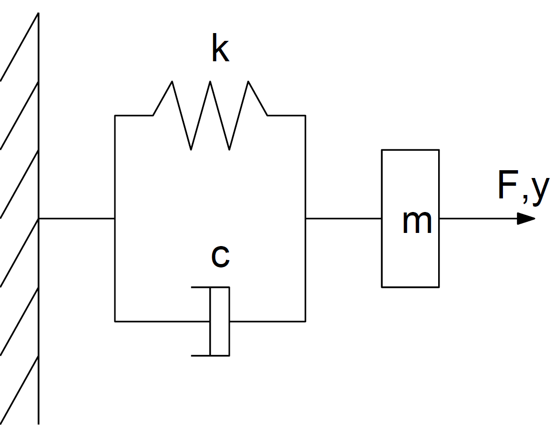
The idea is here to run a numerical simulation of a system with known behavior in order to check that you understand how to used basic tools : time integration, differences between the continuous and discrete Fourier transform, properties of the basic oscillator.

2.1  Free response and FFT

Questions :

• 1. Write the state space model associated with a spring mass system with M = 1, K=4e2
• 2. Choose C to have a damping ratio of 1 % (tip : you need to compute eigenvalues of the state matrix A at see the ration between the real part and the amplitude of poles)
• 3. Use a time integration function ode45 (in the engine cover application, we will also use lsim which is faster but only works for LTI systems), to compute the response to a non zero initial condition. Plot this response.
• 4. Chooze a time interval and compute the Fourier transform (using fft). Find the resonance frequency and in this FFT (compute the frequencies from the time vector).
• 5. Illustrate the influence of the damping ration by overlaying the fft for three distinct values of C.

Programming suggestions

% Create your deriv function which will have (t,y,PA) as inputs
% Store all parameters in a structure
PA=struct('A',[],'B',[],'u',[]);
 [t,y]=ode45(@deriv,tspan,y0,odeset,PA)
% Use t,y for time, F,Y for frequency response

% Damping study, store multiple results as a structure, then finalize plot
damp=[ ??? ];
C1=struct('X',[],'Y',[]); % prepare structure for result
for j1=1:length(damp)
 ???
 C1.X=f; C1.Y(:,j1)=Y(:,1); % store first column for each result in loop
end

% Finalize plot
plot(C1.X,C1.Y);xlabel('x');ylabel('y');set(gca,'xlim',[0 50])

2.2  Forced response

Questions :

1. Apply a sinusoidal force (choose the amplitude and frequency) and illustrate how the corresponding frequency appears in the fft of the response.
2. Illustrate windowing issues by keeping an integer/non-integer number of periods, in other words, a frequency that exists/does not exist in the spectrum.
3. Illustrate how the transient decreases and depends on initial conditions. (Tip : compare fft for a full signal or a signal starting at T>0).
4. Illustrate Shannon's theorem by using an excitation above the half sampling frequency (spectrum symmetry point).

Programming suggestions

% Forced response
PA.u=@(t)sin(10*t); % Define an "anonymous" function for response
% Truncate the first 10 s
ind=(t>10);t=t(ind);y=y(ind,:); 

2.3  Non-linear response

One now considers the classical cubic non-linearity (even if this rarely corresponds to something mechanical)

• Apply a sinusoidal force. What frequencies are seen in the response fft ?
• How does the response at harmonics of the excitation frequency vary with amplitude (or the α coefficient).

α=10⁻⁶ is a decent starting value. Pay attention to the need to eliminate the transient associated with the initial condition.

2.4  Sweep excitation

One considers an excitation through a swepped sine

 PA=struct('A', ??? ,'B',[0;1],'u',[]); % Adjust damping here
 fmin=15;fmax=25;PA.u=@(t)cos((fmin+(fmax-fmin)/2*t/tspan(end))*t);  % Sweep

• In the time response, how is the resonance visible ?
• How does the variance (var) change with damping ?